Mode Shapes and Frequency Response

This experiment uses two accelerometers to measure the frequency response of a scaled three-story flexible structure and a helicopter blade using a digital scope and network analyzer performing a sinusoidal excitation, beginning at a lower frequency and increasing over time. The phase shift between the two accelerometers and the anti-resonance and resonance modes are calculated and compared to visually confirmed resonance modes for the three-story structure and finite element analysis (FEA) modeled resonance modes for the helicopter blade respectively.
In our laboratory experiment, we conducted a comprehensive analysis of the vibration modes on a model three-story building and a model helicopter blade using a sine sweep. The utilization of this method enabled us to excite a wide range of frequencies, which helped us to identify different resonance and anti-resonance modes of our structures. By deriving analytical transfer functions for these modes, we were able to gain a better understanding of the underlying dynamics of the structures.
Understanding the resonance and anti-resonance frequencies is critical to designing any component expected to experience and withstand vibrational forces, given that at their resonance frequencies forces are compounded on top of each other and typically lead to catastrophic failure.
Background Theory: Lagrange’s method, Ordinary Differential Equations, Linear System Theory, mass, damping and stiffness matrices, mode shapes
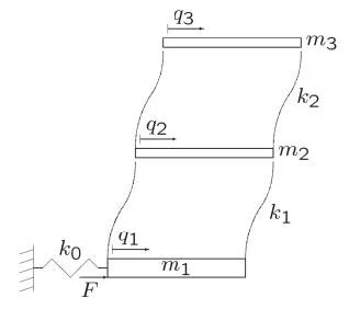
Schematic of simple spring-loaded two-story building subjected to base force excitation
Apparatus

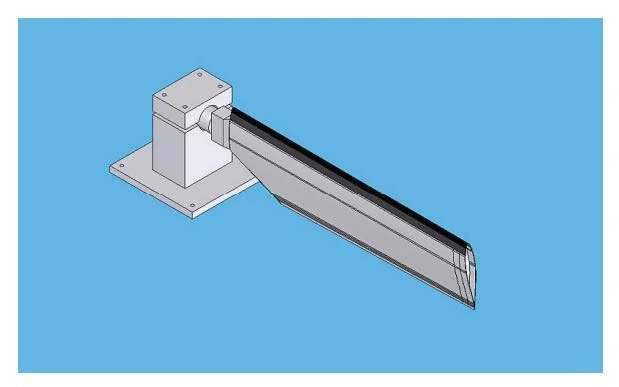
table-top mounted blade of helicopter tail rotor
Network Analysis of Flexible Building Resonance Modes
The mode shape at anti-resonance frequency for each floor is shown in the figure below. The performance of the vibration at different frequencies can be easily observed by transfer functions.
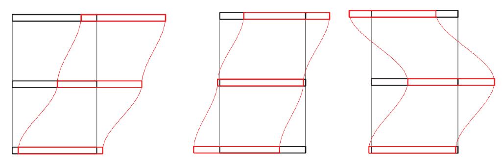
Mode shapes. From left to right: 1st mode, 2nd mode, 3rd mode
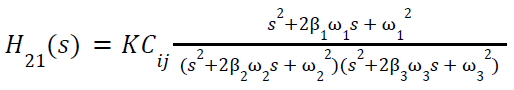
The frequency response of the three-story building can be modeled as a transfer function to predict how the building will react.
with ω2 and ω3 being the resonance frequencies and ω1 is the anti-resonance frequency.
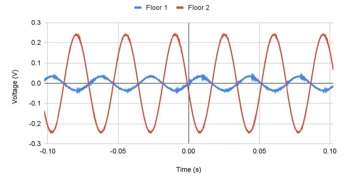
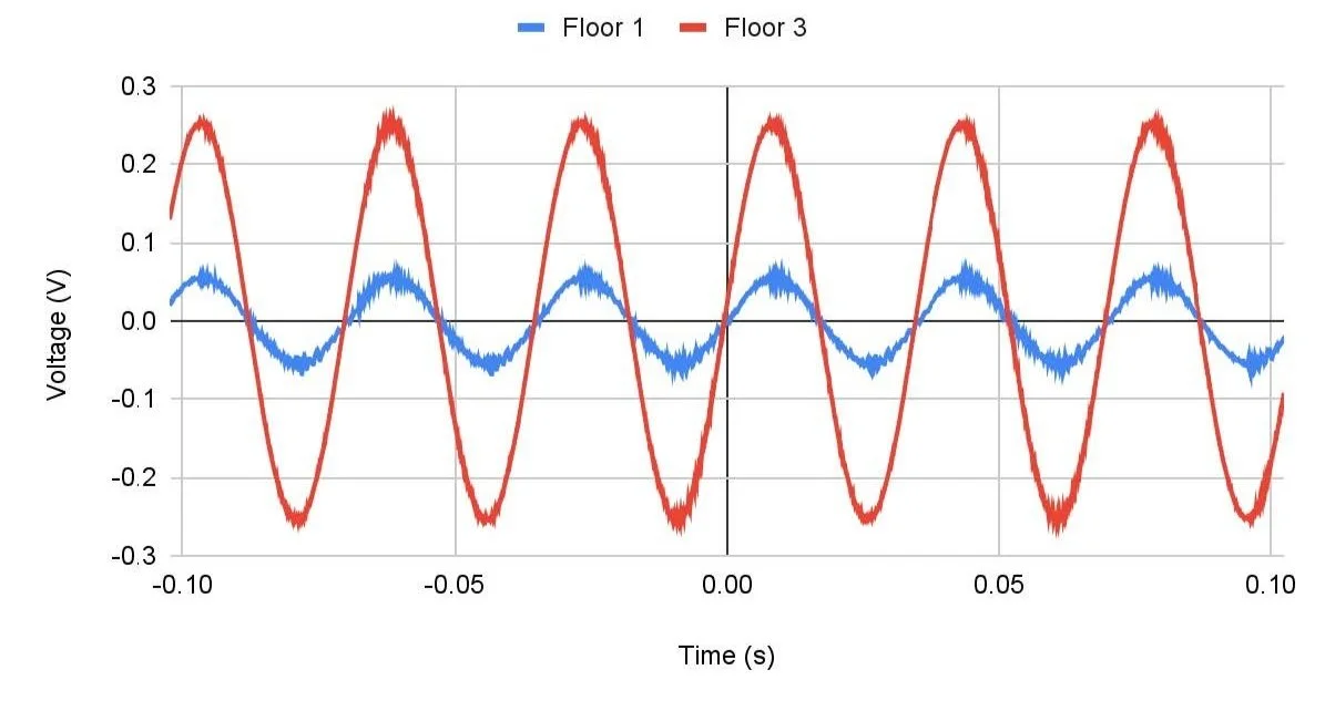
From the accelerometers, voltage data was gathered and graphed to measure the response of each floor to the oscillations. Visually, mode frequencies were determined to be 8.9, 12.9, and 28.6 Hz for modes 1, 2, and 3 respectively.
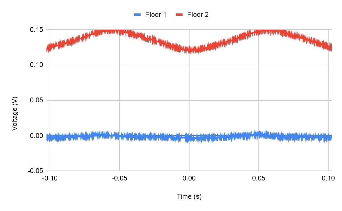

Frequency Response at 8.9 Hz
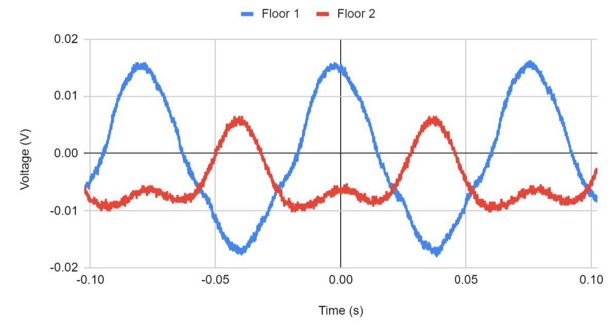
Frequency Response at 12.9 Hz
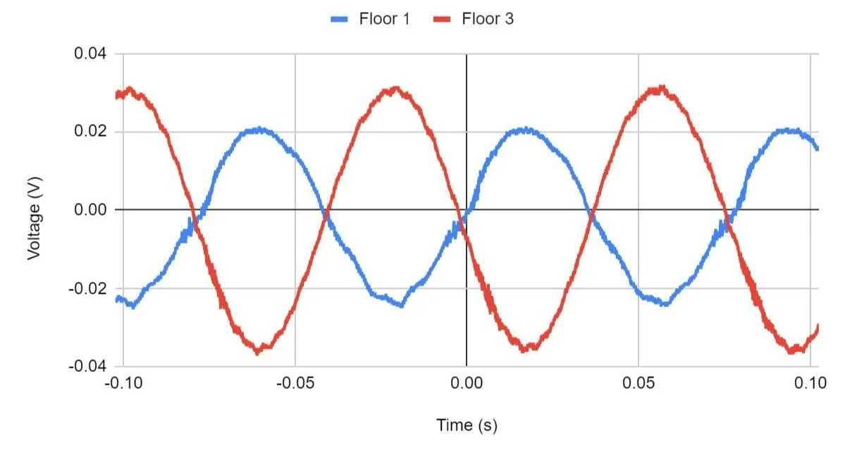
Frequency Response at 28.6 Hz
The bode plot below shows that the resonance frequencies from floors 1 and 2 were 8.9 Hz and 27.9 Hz, while the anti-resonance frequency was 14.4 Hz.
The dampening of the model was tuned to β1 =0.2, β2 =0.01, β3 =0.05
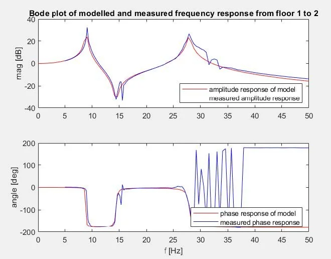
Bode plot of the measured and modeled frequency response from floors 1 and 2
The bode plot below shows that the resonance frequencies from floors 1 and 3 to be 9.1 Hz and 27.9 Hz while the anti-resonance frequency was 12.4 Hz.
The dampening of the model was tuned to β1 =0.01, β2 =0.005, β3 =0.01
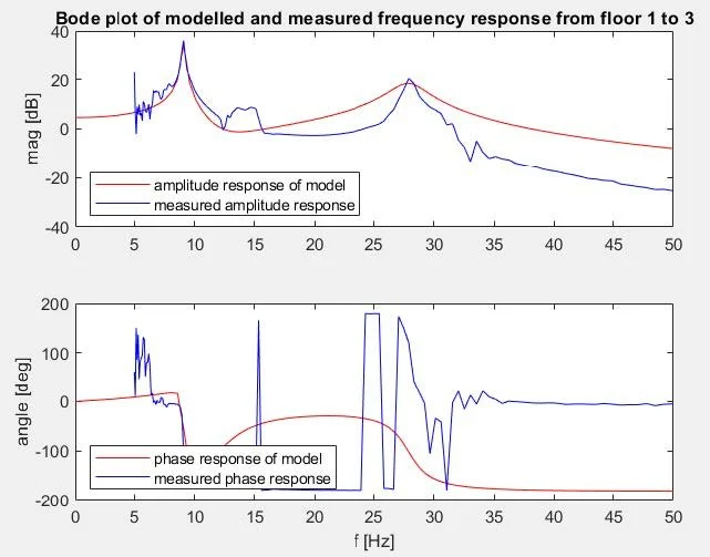
Bode plot of the measured and modeled frequency response from floors 1 and 3
There are several reasons why our simulated and experimental results were different. For example, in the ideal simulation of a 3-story building, all three floors are assumed to move parallel to each other and be perfectly level, which may not reflect reality. Additionally, the shaker table used in the experiment is not a perfectly ideal spring, and some energy is likely lost to heat, which can offset the energy balance. Furthermore, external vibrations and noise from the environment can affect the accuracy of the accelerometers used to collect experimental data. Resistance from the wires connecting the accelerometers to the data acquisition system as well as the gum adhering the accelerometer to the measured surface are a couple of environmental conditions that could be held responsible for causing deviations from the simulated results.
Network Analysis of Helicopter Blade
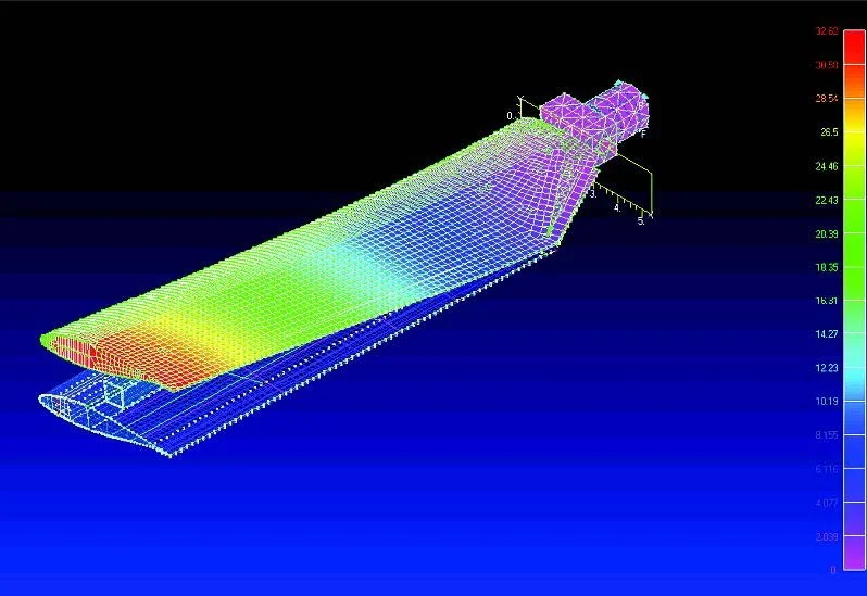
1st mode: out-of-plane bending
Courtesy of Prof. J. Kosmatka, Dept. of Structural Engineering, UCSD
The plot shows the out-of-plane resonance frequencies of the wing to be 50.9 Hz and 94 Hz while the anti-resonance frequency is seen as 70 Hz. The dampening of the model was tuned to β1 =.2, β2 =.001, and β3 =.1

Bode plot of the measured and modeled out-of-plane frequency response of the wing

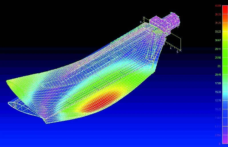
2nd mode: ‘in-plane’ bending
Courtesy of Prof. J. Kosmatka, Dept. of Structural Engineering, UCSD
The plot shows the in-plane resonance frequencies of the wing to be 56.9 Hz and 152.9 Hz while the anti-resonance frequency is seen as 83 Hz. The dampening of the model was tuned to β1 =.11, β2 =.09, and β3 =.001
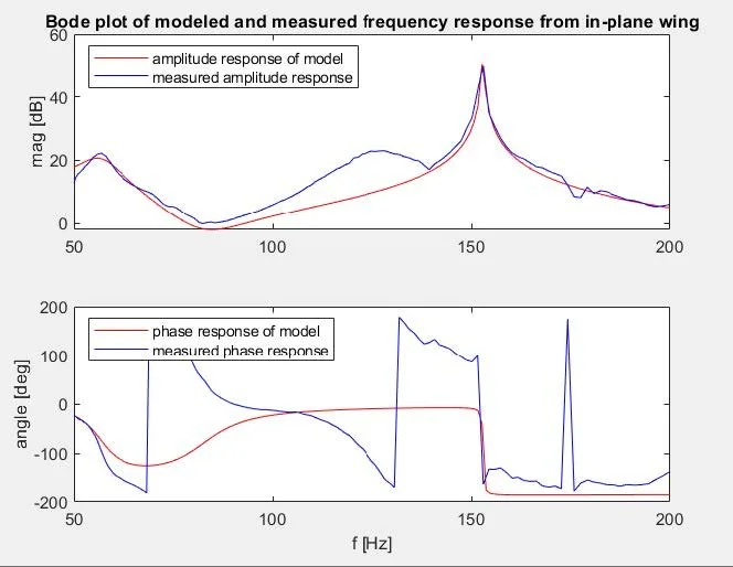
Bode plot of the measured and modeled in-plane frequency response of the wing
3rd mode: torsion mode
Courtesy of Prof. J. Kosmatka, Dept. of Structural Engineering, UCSD
The plot shows the torsion resonance frequencies of the wing to be 87.8 Hz and 175 Hz while the anti-resonance frequency is seen as 157.3 Hz. The dampening of the model was tuned to β1 =.02, β2 =.02, and β3 =.03

Bode plot of the measured and modeled torsion frequency response of the wing